Linear and Logistic Regression, Part 2: Fitting the Models

By Colby Roberts on December 21, 2020

Note: This post is part 2 of a 3-part series: part 1, part 2, part 3.

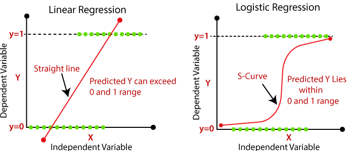
This is a blog post exploring how to fit linear and logistic regressions. First, note that linear and logistic regressors have different shapes. The shape of linear regression is a line, while the shape of logistic regression is a sigmoid:

Also note that the same procedure can be used to fit a linear or logistic regressor, because the logistic equation can be rearranged to become a linear one.

Linear Function	Logistic Function
$\beta_0 + \beta_1 x_1 + \ldots + \beta_n x_n=y$	$\begin{align} \dfrac{1}{1+e^{\beta_0 + \beta_1 x_1 + \ldots + \beta_n x_n}}&=y \\ \beta_0 + \beta_1 x_1 + \ldots + \beta_n x_n &= \ln\left(\dfrac{1}{y}-1\right) \end{align}$

Let $y^\prime = y$ for the case of a linear regression, and $y^\prime = \ln\left(\dfrac{1}{y}-1\right)$ for the case of a logistic regression. Then, we need to fit the regression to the following dataset:

$\begin{align*} \left\{ \begin{matrix} (x_{11}, & x_{12}, & \ldots & x_{1n}, & y_1^\prime) \\ (x_{21}, & x_{22}, & \ldots & x_{2n}, & y_2^\prime) \\ \vdots & \vdots & \ddots & \vdots & \vdots \\ (x_{m1}, & x_{m2}, & \ldots & x_{mn}, & y_m^\prime) \end{matrix} \right\} \end{align*}$

So, we need to solve the matrix equation

$\begin{align*} \begin{pmatrix} 1 & x_{11} & x_{12} & \ldots & x_{1n} \\ 1 & x_{21} & x_{22} & \ldots & x_{2n} \\ \vdots & \vdots & \vdots & \ddots & \vdots \\ 1 & x_{m1} & x_{m2} & \ldots & x_{mn} \end{pmatrix} \begin{pmatrix} \beta_0 \\ \beta_1 \\ \vdots \\ \beta_m \end{pmatrix} &\approx \begin{pmatrix} y_1^\prime \\ y_2^\prime \\ \vdots \\ y_m^\prime \end{pmatrix}. \end{align*}$

We can put this in equation form and perform operations to isolate $\vec{\beta}\mathbin{:}$

$\begin{align*} \mathbf{X} \vec{\beta} &\approx \vec{y}\\ \mathbf{X} \vec{\beta} &\approx \vec{y} \\ \mathbf{X}^T \mathbf{X} \vec{\beta} &\approx \mathbf{X}^T \vec{y} \\ \vec{\beta} &\approx \left( \mathbf{X}^T \mathbf{X} \right)^{-1} \mathbf{X}^T \vec{y} \end{align*}$

This way of finding $\vec{\beta}$ involves using the pseudoinverse, $\left( \mathbf{X}^T \mathbf{X} \right)^{-1} \mathbf{X}^T.$ A matrix is not invertible unless it is square and we cannot guarantee this for $\mathbf{X},$ so we must take the pseudoinverse. By multiplying a $\mathbf{X}$ by its transpose, we can ensure that the result is square, and therefore, we can compute the inverse. Using the pseudoinverse minimizes the sum of squared error between the desired output $\vec{y}$ and the actual output $\mathbf{X}\vec{\beta}.$

For example, let’s fit a logistic regression to a medical data set

$\begin{align*} [(0, 0, 0.1), (1, 0, 0.2), (0, 2, 0.5), (4,5,0.6)] \end{align*}$

which takes the form

$\begin{align*} (\textrm{amount medicine A}, \textrm{amount medicine B}, \textrm{survival probability}). \end{align*}$

This data set is for a new medicine where the first column shows the amount of medicine A and the second medicine B. We have data on how well these medicines did when given to patients in differing amounts.

We can fit a logistic regression as follows:

$\begin{align*} \mathbf{X} = \begin{pmatrix} 1 & 0 & 0 \\ 1 & 1 & 0 \\ 1 & 0 & 2 \\ 1 & 4 & 5 \end{pmatrix} \ \ \& \ \ \vec{y} = \begin{pmatrix} \ln \left( \dfrac{1}{0.1} - 1 \right) \\ \ln \left( \dfrac{1}{0.2} - 1 \right) \\ \ln \left( \dfrac{1}{0.5} - 1 \right) \\ \ln \left( \dfrac{1}{0.6} - 1 \right) \end{pmatrix} = \begin{pmatrix} \ln \left( 9 \right) \\ \ln \left( 4 \right) \\ \ln \left( 1 \right) \\ \ln \left( \dfrac{2}{3} \right) \end{pmatrix} \end{align*}$

$\begin{align*} \vec{\beta} &\approx (\mathbf{X}^T \mathbf{X})^{-1} \mathbf{X}^T \vec{y} \\ \vec{\beta} &\approx \left(\begin{pmatrix} 1 & 1 & 1 & 1\\ 0 & 1 & 0 & 4 \\ 0 & 0 & 2 & 5 \end{pmatrix} \begin{pmatrix} 1 & 0 & 0 \\ 1 & 1 & 0 \\ 1 & 0 & 2 \\ 1 & 4 & 5 \end{pmatrix}\right)^{-1} \begin{pmatrix} 1 & 1 & 1 & 1\\ 0 & 1 & 0 & 4 \\ 0 & 0 & 2 & 5 \end{pmatrix} \begin{pmatrix}\ln \left( 9 \right) \\ \ln \left( 4 \right) \\ \ln \left( 1 \right) \\ \ln \left( \dfrac{2}{3} \right)\end{pmatrix} \\ \vec{\beta} &\approx \begin{pmatrix} 4 & 5 & 7 \\ 5 & 17 & 20 \\ 7 & 20 & 29 \end{pmatrix} ^{-1} \begin{pmatrix} 1 & 1 & 1 & 1\\ 0 & 1 & 0 & 4 \\ 0 & 0 & 2 & 5 \end{pmatrix} \begin{pmatrix}\ln \left( 9 \right) \\ \ln \left( 4 \right) \\ \ln \left( 1 \right) \\ \ln \left( \dfrac{2}{3} \right)\end{pmatrix} \\ \vec{\beta} &\approx \begin{pmatrix} 1.567 \\ 0.278 \\ -0.640 \end{pmatrix} \end{align*}$

Now we know the logistic $\beta$’s which are $\beta_0 = 1.567 \ \& \ \beta_1 = 0.278 \ \& \ \beta_2 = -0.640,$ so we plug in the variables $x_1, \ \& \ x_2$ into the equation:

$\begin{align*} f(x_1,x_2) &=\dfrac{1}{1 + e ^ {\beta_0 + \beta_1 x_1 + \beta_2 x_2}} \\ &=\dfrac{1}{1 + e ^ {1.567 + 0.278 x_1 -0.640 x_2}} \end{align*}$

Because very little changes from the linear regressor to the logistic regressor, my Python code for the logistic regressor inherits from the linear regressor class and changes only 2 things: it transforms the $\vec{y}$ using $y’ = \ln \left( \dfrac{1}{y}-1 \right)$ and puts the $\beta$’s in a sigmoid function rather than a linear function.

First, let’s go through the code for the linear regressor. We start by importing a Matrix class and a Dataframe class that I had written to help process data. Then, we initialize the linear regressor:

from matrix import Matrix
from dataframe import DataFrame
import math

class LinearRegressor:
    def __init__(self, dataframe, dependent_variable='ratings'):
        self.dependent_variable = dependent_variable
        self.independent_variables = [column for column in dataframe.columns if column != dependent_variable]
        X_dataframe = dataframe.select.columns(self.independent_variables)
        y_dataframe = dataframe.select_columns([self.dependent_variable])
        self.X = Matrix(X_dataframe.to_array())
        self.y = Matrix(X_dataframe.to_array())
        self.coefficients = {}

The way we would solve to get the $\vec{\beta}$’s is as follows:

    def solve_coefficients(self):
        beta = (((self.X.transpose() @ self.X).inverse()) @ self.X.transpose()) @ self.y
        self.set_coefficients(beta)

    def set_coefficients(self, beta):
        for i, column_name in enumerate(self.dependent_variables):
            self.coefficients[column_name] = beta[i]

In order to find the actual prediction that the regression with the $\beta$’s, we need to plug the $\beta$’s into the regression function. For the linear regressor, this is just a linear function $f(x_1,\ldots, x_n)=\beta_0 + \beta_1 x_1 + \ldots + \beta_n x_n.$

    def predict(self, input_dict):
        return self.regression_function(input_dict)

    def regression_function(self, input_dict):
        return sum([input_dict[key] * self.coefficients[key] for key in input_dict])

For the logistic regression, it’s the same process but we need to transform the $y$ values:

class LogisticRegressor(LinearRegressor):
    def __init__(self, dataframe, dependent_variable='ratings'):
        super().__init__(dataframe, dependent_variable='ratings')
        self.y = self.y.apply(lambda y: math.log(1/y - 1))

And we use a different regression function:

$\begin{align*} f(x_1,\ldots, x_n)=\dfrac{1}{1+e^{\beta_0 + \beta_1 x_1 + \ldots + \beta_n x_n}} \end{align*}$

    def regression_function(self, input_dict):
        linear_sum = sum([gathered_inputs[key] * coefficients[key] for key in gathered_inputs])
        return 1 / (1 + math.e ** linear_sum)

This post is part 2 of a 3-part series. Click here to continue to part 3.

Colby Roberts is a junior in Math Academy and App Academy at Pasadena High School. He plays on the PHS Football team, loves coding and and gaming, and is in Chess Club. He is a true nerd who spends 99% of his money on better PC parts for the computer he built. In college, Colby wants to study computer science. Last updated 2020.

-->