Predator-Prey Modeling with Euler Estimation

By David Gieselman on December 21, 2020

Predator-prey relationships are common in nature. One species benefits from a high population of the other, while the other species is hurt by a high population of the first species.

An example of this could be two populations of deer and wolves in a closed system. When the deer population is high, the rate of the wolf population grows because their food source is abundant. However, the more wolves there are, the more deer are eaten, and the fewer deer there are. So the population sizes alternate between the variables which results in a consistent oscillation.

Below is a simple example of a system of equations in a predator-prey model.

$\begin{align*} \begin{cases} \dfrac{\text{d}D}{\textrm{d}t} = (0.6) D + (-0.05) DW, \quad D(0) = 100 \\[10pt] \dfrac{\text{d}W}{\textrm{d}t} = (-0.9) W + (0.02) DW, \quad W(0) = 10 \\ \end{cases} \end{align*}$

In the equations, $D$ represents the deer population and $W$ represents the wolf population. Each term can be interpreted as follows:

$(0.6)D\mathbin{:}$ The deer can increase their population at a rate of $60\%$ when removed from the wolves.
$(-0.05) DW\mathbin{:}$ The wolves kill the deer $50\%$ percent of the time of the wolves interact with the deer, which is at a rate of $0.1$ times per wolf per deer, per year. $DW$ represents the deer-wolf interaction because as each population increases, interaction increases because of more crowding in the environment.
$(-0.9)W\mathbin{:}$ Removed from the deer, the wolves die off at a rate of $90\%$ per year.
$(0.02)DW\mathbin{:}$ The wolf population increases by $0.4$ per eaten deer.

To get a graph of the populations compared to each other, we can use Euler estimation.

Euler estimation works by taking a starting point and using a differential equation to repeatedly predict where it will go. Each iteration, we use the differential equation to estimate the slope of the line at the starting point and move the starting point along that slope. This works because the derivatives in the differential equation are the rates of change.

In the case of the wolf deer system, the derivatives are presented in the system of equations above. The given values $D(0)=100$ and $W(0)=10$ are the starting points when the time (in years) was 0.

Here, the Euler estimation can be shown mathematically like so:

$\begin{align*} D(t+\Delta t)&\approx D(t)+D ^\prime (t)\Delta t \\ W(t+\Delta t)&\approx W(t)+W ^\prime (t)\Delta t, \end{align*}$

where $D^\prime$ and $W^\prime$ are the derivatives of $D$ and $W$ and $t+\Delta t$ represents the change along the timeline in accordance to the step size $\Delta t.$ Specificity can be increased by making $\Delta t$ smaller.

These equations for $D$ and $W$ take the same form, because this just a general Euler estimation formula. The difference in math comes from their differing differential equations in the original system.

For example, if we began working out the deer-wolf model with a step size of $\Delta t = 0.1$ by hand, the first step would look like so:

$\begin{align*} D(0.1) & =D(0)+D ^\prime (0) * 0.1\\ &=100-10 * 0.1\\ &=99 \\ \\ W(0.1)&=W(0)+W ^\prime (0) * 0.1\\ &=10+11 * 0.1\\ &=11.1 \end{align*}$

Here is the next step:

$\begin{align*} D(0.2)&=D(0.1)+D ^\prime (0.1)*0.1\\ &=99+4.455*0.1\\ &=99.4455 \\ \\ W(0.2) &=W(0.1)+W ^\prime (0.1)*0.1 \\ &=11.1+11.98*0.1 \\ &=12.2988 \end{align*}$

If we wanted to get to a $t$ of say, $t=100,$ doing this by hand would take hours. These $2$ steps took me $5$ minutes, and we would need to do it $1000$ times! So, we need to write some code.

In my Euler estimation code, there is a class EulerEstimator with 2 main methods:

calculate_derivative_at_point() - finds how much the equation is increasing at a point by plugging it into the differential equation
step_forward(step_size) - is repeated over and over

In the code for step\_forward(step\_size), the derivative is multiplied by the step size and added to each of the $y$ variables.

derivative_at_point = calc_derivative(point)
num_coordinates = len(derivative_at_point)
new_point = []
for coordinate_index in range(num_coordinates):
    derivative_entry = derivative_at_point[coordinate_index]
    point_entry = point[coordinate_index]
    new_point.append(point_entry + step_size * derivative_entry)

The graph below shows the plot of the Euler estimation of the wolf and deer populations.

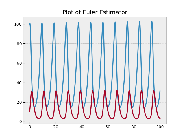
The populations both oscillate. As the wolf population rises, they kill more deer. Then, as the deer population falls, the wolves starve and their population decreases. With the scarcity of wolves, the deer thrive and their population booms and the cycle begins again.

Note that the step size is an important part of Euler estimation. Having a small step size will give you more accurate results, but will add to computation time and may be more accurate than necessary. However, having too large of a step size can make the simulation too inaccurate. It reduces the amount of computation, but also reduces the amount of detail. It’s kind of like resolution on a monitor: you want it to be enough so that your eyes can make out what’s happening, but you don’t want it to take too much time to compute.

David Gieselman is a junior in Math Academy and App Academy at Pasadena High School. David plays for the PHS football team and also runs track. In his free time, David likes to play video games, practice graphic design, and listen to music. He is also working to get his Eagle Scout rank in boy scouts. David plans on studying aerospace engineering in college. Last updated 2020.

-->