Simulating a Biological Neuron Using the Hodgkin-Huxley Model

By Justin Hong on June 01, 2021

To understand the Hodgkin-Huxley model, we must first understand what a neuron is. A neuron is a type of cell that is most prominently found in nerves and the brain, and neurons the primary building blocks of the nervous system. Neurons are connected by synapses, which allow signals to be sent and received rapidly and precisely.

There are three major types of neurons:

Sensory neurons make sense of the outside world (e.g. touch, pain, vision, hearing, and taste) by sending signals from sensory organs to the brain.
Inter-neurons make up most of the neurons in our bodies and brain, and allow us to to think, see, and perceive things.
Motor neurons are in charge of contracting muscles so we can move.

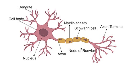
The most basic structure of a neuron consists of the main cell body (the plasma membrane, nucleus, etc.), dendrites, and an axon. Dendrites allow the neuron to receive signals, while the single axon is how the cell sends signals.

Neurons send signals via spikes in electrical activity called action potentials. Before we jump into modeling action potentials, let’s learn a bit more about them.

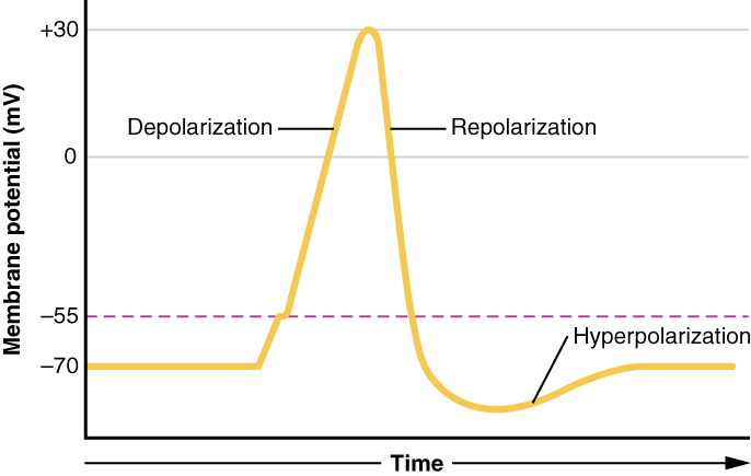
Each neuron has a resting membrane potential around -70 mV (it is negative because the surroundings of the neuron have accumulated ions). As neurotransmitters bind to the receptors, the neuron is depolarized, moving the membrane potential closer to 0 mV. When the membrane potential reaches a certain threshold (around -55 mV for a neuron starting at -70 mV), sodium channels open, allowing many sodium ions into the cell. Rapid depolarization follows, and the membrane potential becomes positive. This influx of positive charge is what is known as the action potential.

When the action potential reaches its peak, sodium channels close, potassium channels open, and the cell loses membrane potential (repolarization). The drop in membrane potential causes the neuron to become hyperpolarized, and enter a state where it is very difficult to cause the neuron to depolarize again. Eventually the neuron reaches its resting membrane potential again, where it is no longer hyperpolarized.

The Hodgkin-Huxley Model

The Hodgkin-Huxley model won the Nobel Prize in 1963 for Physiology and Medicine, and the prize was awarded to Sir John Carew Eccles, Alan Lloyd Hodgkin, and Andrew Fielding Huxley. These men won the prize for their model of the action potentials of neurons using differential equations.

The model yields a graph of how electrical stimulus affects the action potential (change in voltage) of a neuron over time. Hodgkin and Huxley derived much of the model from experimentation, and those results combined with physics to yield usable differential equations.

From physics, we have that the current is proportional to the change in voltage via the capacitance

$\begin{align*} I = C \dfrac{dV}{dt}, \end{align*}$

and from this we can obtain

$\begin{align*} \dfrac{dV}{dt} = \dfrac{I}{C}. \end{align*}$

In neurons, the capacitance is roughly $1$.

Next the current must be split into parts: the stimulus ($s$), the flux across the sodium and potassium channels ($I_{Na}$, $I_{K}$ respectively), and the current leakage ($I_{L}$). We then turn the previous equation into

$\begin{align*} \dfrac{dV}{dt} = \dfrac{1}{C} \left[ s - I_{Na} - I_{K} - I_{L} \right]. \end{align*}$

In this model it’s really just

$\begin{align*} \dfrac{dV}{dt} = s - I_{Na} - I_{K} - I_{L}. \end{align*}$

since $C=1.$

One thing to keep in mind for all of these equations is that $V$ represents voltage offset from the resting potential (-70 mV), and not the actual voltage of the neuron. This is done to make graphing and showing the model more simple.

The current across each channel (including the leakage) is related to the voltage difference relative to that channel’s equilibrium voltage. The proportionality constants were modeled experimentally, and some are written in terms of $n, m,$ and $h,$ which represent the probability of active/inactive channels. The equations can be written as follows (with $V$ representing voltage offset from the resting potential):

$I_{Na}(V, m, h) = g_{Na}(m,h)(V-V_{Na})$, with equilibrium voltage $V_{Na} = 115$ and proportionality constant $g_{Na}(m,h) = 120m^{3}h$
$I_{K}(V, n) = g_{K}(n)(V-V_{K})$, with $V_{K} = -12$ and $g_{K}(n) = 36n^{4}$
$I_{L}(V) = 0.3(V-V_{L})$, with $V_{L}=10.6$

These variables $n, m,$ and $h$ still have to be dealt with. The rates of change for these variables depends on functions of voltage (alphas and betas), and are written as so:

$\begin{align*} \dfrac{\text dn}{\text dt} &= \alpha_n(V) (1-n) - \beta_n(V) n \\ \dfrac{\text dm}{\text dt} &= \alpha_m(V)(1-m) - \beta_m(V) m \\ \dfrac{\text dh}{\text dt} &= \alpha_h(V) (1-h) - \beta_h(V) h \end{align*}$

The alpha and beta functions are shown here:

$\begin{align*} \alpha_n(V) &= \dfrac{0.01(10-V)}{\exp \left[ 0.1 (10-V) \right] - 1}, \quad& \alpha_m(V) &= \dfrac{0.1(25-V)}{\exp \left[ 0.1 (25-V) \right] - 1}, \quad& \alpha_h(V) &= 0.07 \exp \left[ -\dfrac{V}{20} \right], \\ \beta_n(V) &= 0.125 \exp \left[ -\dfrac{V}{80} \right], \quad& \beta_m(V) &= 4 \exp \left[ - \dfrac{V}{18} \right], \quad& \beta_h(V) &= \dfrac{1}{\exp \left[ 0.1( 30-V) \right] + 1}. \end{align*}$

In this particular example, the stimulus will be provided to the neuron at certain intervals

$\begin{align*} s(t) = \begin{cases} 150, & t \in [10,11] \cup [20,21] \cup [30,40] \cup [50,51] \cup [53,54] \\ & \phantom{t \in [} \cup [56,57] \cup [59,60] \cup [62,63] \cup [65,66] \\ 0 & \text{otherwise}. \end{cases} \end{align*}$

Lastly, initial values must be dealt with. We have $V_{0} = 0$ (remember, $V$ represents the offset from the resting membrane potential), and $n_0, m_0, h_0$ can be approximated with by setting $V = 0$ and setting each $n, m, h$ to their asymptotic values:

$\begin{align*} n_0 &= \dfrac{\alpha_n(V_0)}{\alpha_n(V_0) + \beta_n(V_0)} \\ m_0 &= \dfrac{\alpha_m(V_0)}{\alpha_m(V_0) + \beta_m(V_0)} \\ h_0 &= \dfrac{\alpha_h(V_0)}{\alpha_h(V_0) + \beta_h(V_0)} \end{align*}$

Simulating a Hodgkin-Huxley Neuron

Creating the Hodgkin-Huxley model through code first requires a class or function (using the Python coding language in this case) that is able to create graphs with just differential equations. Euler estimation is the method that is used to do just that. At its very core, the Euler estimator takes the rate of change of a function at a point and predicts the next point based on that rate of change and the user-inputted step size (rate of change times step size gives us the change from the original point to the next point). As the step size decreases, the graph becomes more accurate.

For the Euler estimator used in this case, the user inputs rates of change for each dependent variable, and uses that to calculate the variables needed to graph. Point output is in the form $(t,x),$ where $t$ represents time and $x$ can represent multiple dependent variables via Python dictionary. The estimator will graph time vs. each dependent variable.

All that is left to do is turn the differentials and functions into Python functions, and use the Euler estimator to graph the model.

Here are some examples of turning the equations into code. There is one Python function for every “part” of the model: alphas and betas, initial values, currents, etc.

def alpha_n(t,x):
    V = x['V']
    return (0.01*(10-V)) / (math.exp(0.1*(10-V)) - 1)

n_0 = alpha_n(0,{'V':0}) / (alpha_n(0,{'V':0}) + beta_n(0,{'V':0}))

def I_Na(t,x):
    V = x['V']
    m = x['m']
    h = x['h']
    return 120*(m**3)*h*(V - V_Na)

def stim(t):
    if 10<=t<=11 or 20<=t<=21 or 30<=t<=40 or 50<=t<=51 # (etc)
        return 150
    return 0

def dV_dt(t,x):
    s = stim(t)
    Na_curr = I_Na(t,x)
    K_curr = I_K(t,x)
    L_curr = I_L(t,x)
    return (1/C) * (s - Na_curr - K_curr - L_curr)

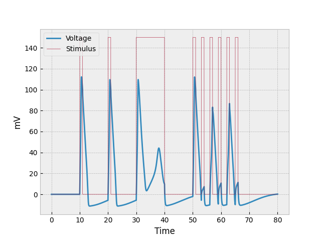
The end product looks something like this:

Analyzing the Model

Now that we have the actual model, we can analyze how it relates to all the information about neurons above, as well as what the model could imply.

If we look at the first burst of stimulus (between $t=10$ and $t=11$), we can see the most basic reaction to stimulus: a sudden spike caused by both depolarization and the stimulus provided (two factors), a more gradual decrease in voltage as the repolarizes (it’s slower than the increase because there is only one factor repolarizing the neuron), and then where the neuron becomes hyperpolarized. This occurs at both $t=20$ and $t=30$ as well, but the example for $t=30$ will be discussed in the following paragraph.

The prolonged stimulus between $t=30$ and $t=40$ causes something interesting to occur in the neuron. The first thing to be noticed is that the neuron initially repolarizes at a slower rate. This is due to constant voltage being added into the system while the neuron is repolarizing. The reason the voltage doesn’t keep going down is because it about reaches the threshold where the cell can once again depolarize (-55 mV, which would be represented as 15 mV on the graph). The odd half-spike that starts around $t=33$ is the second thing to be analyzed. The reason the voltage through the neuron does not increase as quickly as previous increases is because the neuron is still repolarizing (losing voltage) as the stimulus is providing voltage. And the little spike eventually reaches the point where sodium channels just all close, and depolarization stops.

The example shown in the preceding paragraph shows what happens when stimulus is constantly being poured into the system. But what happens when stimulus is provided in many short bursts? This question can be answered by analyzing the neuron’s behavior at $t = 50, 53, 56, 59, 62, 65$. The first burst of stimulus looks normal, but since the second burst of stimulus came before the neuron could properly repolarize (and while it was hyperpolarized), the amount of depolarization was very low. The next burst of stimulus (third one) got a better reaction because the neuron was less hyperpolarized, but it was still less than what we would normally expect. The fourth and sixth bursts are similar to the second, and the fifth one to the first and third.

Justin Hong is a sophomore in Math Academy and App Academy at Pasadena High School. He is on the water polo and swim teams at PHS, plays some chess, and enjoys skiing during winters. When he has free time, he likes to play video games, sleep in, and wander around the kitchen. After high school, he wants to study something along the lines of software or AI development. Last updated 2020.

-->